Does a Variable Speed Pump Make Sense for You?

Some pumping systems are designed and built to work under consistent operating conditions. They move the same amount of liquid at the same pressure all the time. 

Most systems, however, are anything but steady state. Take, for example, a pump station that handles storm water. It may handle a few million gallons per day most of the time and five to 10 to even 20 times that volume when it rains. In applications where the system head or flow rate will vary over time, variable speed pumping often makes sense.

The most common method to vary pumps speed is with a variable frequency drive (VFD), which changes the speed of an electric motor that is driving a pump. By changing pump speed based on system variables, the system can compensate for changing flow or head requirements. 

Yet the decision to buy a variable speed pump is not always straightforward. It will depend on how variable the system demands are. In some instances, a better (and more economical) solution might involve utilizing multiple constant-speed pumps of varying sizes to operate individually or in parallel to meet the varying system requirements. 

So, do you really need a variable speed pump? Using the engineering approach found in Hydraulic Institute’s Variable Speed Pumping Guidebook, let’s answer some questions to find out.

What is the maximum system flow, and does system flow or head vary? This is the first and most obvious question to ask. Variable speed pumps might make sense in systems that deal with variable flow, like storm water or municipal drinking water, or variable head, such as a complex pumping system whose switches cause system head requirements to rise and fall at different times. 

What does the system curve tell you about these variations? To understand how a system will handle variations in flow or head, you must understand the system head curve. This is because the intersection of the pump curve and system curve will be the system operating flow and head. The system curve can be calculated by physical equations as a function of flow rate. For simple systems, these calculations can be done by hand. For more complex systems, they are typically done with hydraulic modeling software (see www.pumps.org/freetools). Calculating the system head curve serves as the basis of understanding how varying pump speed will change system flow, head, and power consumption. 

To calculate the system curve, you will need to estimate the friction loss characteristics of all the piping and equipment in the system and the elevation and pressure difference between the source and the supply. The liquid flowing through components will create friction head (which increases with velocity). The difference between the source and supply elevation and pressure is static head (which is not velocity dependent). This curve will arc from the top right of the graph (high head/low flow) to the bottom left (low head/high flow), as shown in Figure 1. 

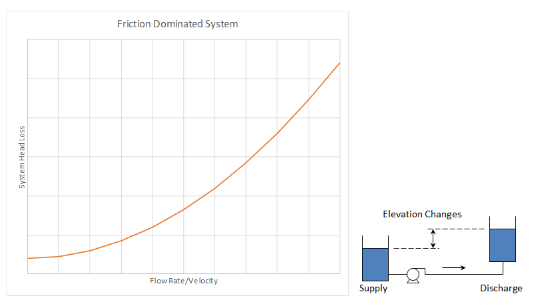
Figure 1 – System curve with predominantly friction head

It is important to consider how the system curve will change over time or by design. Figure 2 shows and example of a system curve that has increased friction head as the piping ages, and how static head will change based on the receiving tank level.

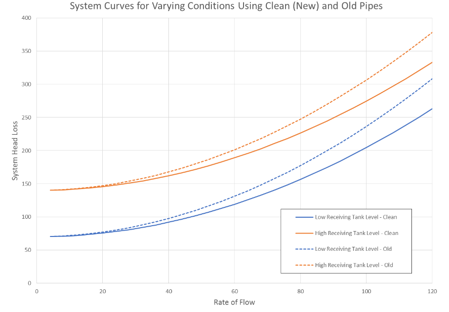
Figure 2 – Varying system curve based on receiving tank level and age.

What pumps meet your maximum operating points? Find one or more pumps that meet the maximum operating flow. We do this by plotting the pump performance curve(s) against the system curve. Where they intersect is the operating flow and head of the system. As shown in Figure 3, a 1780 rpm (full speed) pump that meets the maximum operating flow at a reduced speed of 1580 rpm and the remaining system operating flows at 1325 rpm, 1150 rpm, and 1025 rpm.
 

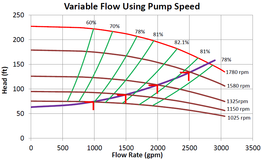
Figure 3 – Pump and system curve intersection is the operating point.

From figure 3 we can see that the system operating flow and head drops as the pump speed declines. The shape of the system (high static head or low static head) will dictate the speed reduction that is possible. We can see that the operating point is cutting across the green efficiency lines as speed is reduced with the higher flow operating to the right of the best efficiency point (BEP), and the lower flows operating to the left of BEP. At the minimum allowable speed of 1025 rpm, the efficiency is 78 percent. If the speed fell below 1025 rpm, the pump efficiency would decline quickly, and the pump head would drop below the system head resulting in no flow to the system. 

Does the normal system operation result in operation within the Preferred Operating Region? Each pump has a preferred operating region (POR) where efficiency and reliability are at their highest. For centrifugal pumps, the POR is typically 70 to 120 percent of the pumps’ best efficiency point. For mixed and axial flow pumps, the POR range is narrower. For example, Figure 3 shows that by utilizing variable speed pumping, each of the operating points (2500, 2000, 1500, and 1000 gpm) lie within the pump’s POR. Employing variable speed pumping allows us to maximizing operating time in the POR, which is a key consideration in pump selection.

What are your alternatives? If your operating envelope does not fall within the pump’s POR, there are alternatives to a single variable speed pump. They include multiple parallel pumps of similar or different sizes that could include one or more variable speed pumps. 

How would that work? Consider, for example, the storm water station mentioned earlier. It may pump 2 MGD on a dry day and 20 MGD on a wet day. That is a 10:1 flow difference. Is there a single pump that could handle this? Probably not. But several pumps operating individually and then in parallel could meet the wide range of flow.

The station might have dry weather 70 to 80 percent of the time, so it makes sense to have a dedicated low-flow pump that runs on those days. When it rains, a medium pump would turn on. For torrential rainfalls, a second medium or even a large pump would kick in.

Using variable speed pumping in combination with parallel pumps can maximize efficiency. The plant could still use a small pump during dry weather. When it rains, a medium-size variable speed pump would come online and raise its speed as inflow increases. At a certain point, a second and even a third variable-speed pump would start up, staged to keep each pump operating in its POR. 

Does life cycle cost (LCC) analysis justify your solution? When analyzing an array of options (constant speed, variable speed, parallel pumps, etc.), a LCC analysis will support which option should be selected. The two largest components of a pump’s LCC is energy and maintenance, typically accounting for 40 percent and 25 percent, respectively. Using variable speed pumping to keep pumps operating in their POR will result in the lowest energy and maintenance costs. These cost savings are balanced against the additional initial and installation cost associated with a VFD, instrumentation, and control logic. 


To learn about analyzing variable speed pumps in greater detail, see Hydraulic Institute’s Variable Speed Pumping Guidebook. 

Subscribe to the Pump Systems Matter Newsletter through out Contact Us form. 

SUBSCRIBE TODAY

Get the latest pump industry news, insights, and analysis delivered to your inbox.

UPCOMING EVENTS